
Classic shock-expansion theory provides the surface pressure of a single body moving through a two-dimensional inviscid continuum fluid at supersonic speeds. Shockwaves are assumed to be infinitely thin and attached so that there are no subsonic regions relative to the body. The flow outside of the shockwaves is assumed to be isentropic, calorically perfect, steady, and irrotational. All wave interactions are assumed to be complete attenuation or amplification, with negligible reflection or transmission. This last assumption in particular is what restricts its range of application to the near-field of single bodies. Inlet flows, supersonic blade cascades, Bussemann biplanes, wing-tail analysis, nozzle flows, supersonic exhaust, far-field sonic booms, formation flying, wind tunnel wall effects; none of these challenging examples can be properly evaluated without modeling the wave interactions.
In this post, I will present my results in attempting to model these wave interactions. I am likely not the first to apply this method and my code is currently far from efficient, but for a limited number of problems, this method could be much faster than Euler based computational fluid dynamics while avoiding some of the problems with shockwaves that the method of characteristics encounters. There will not be much discussion of the math here, but I intend to one day write another post that goes into much more detail when I have rewritten my code. For now, I have selected three cases to present.
Case 1: The Supersonic Ramp Step
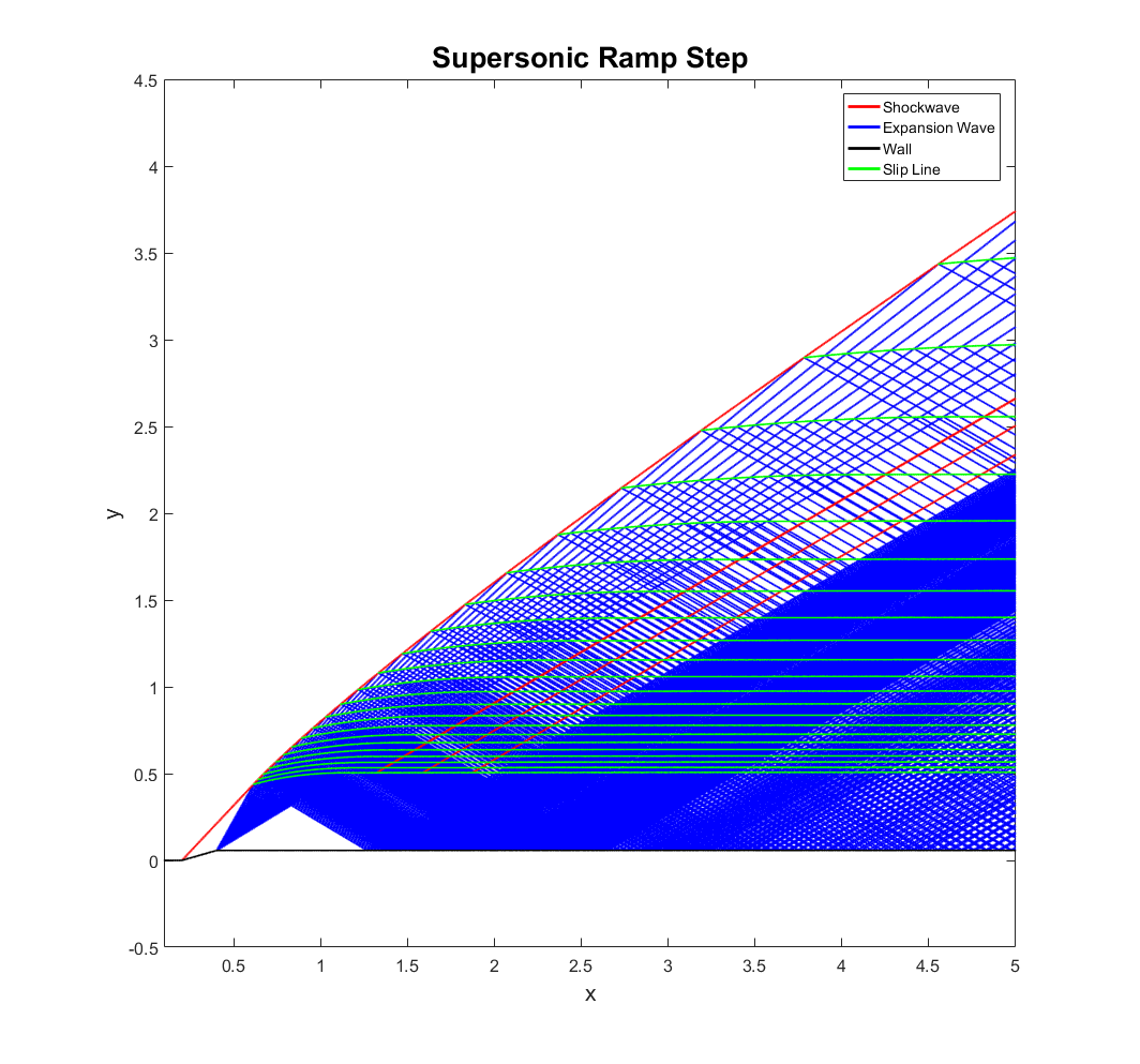
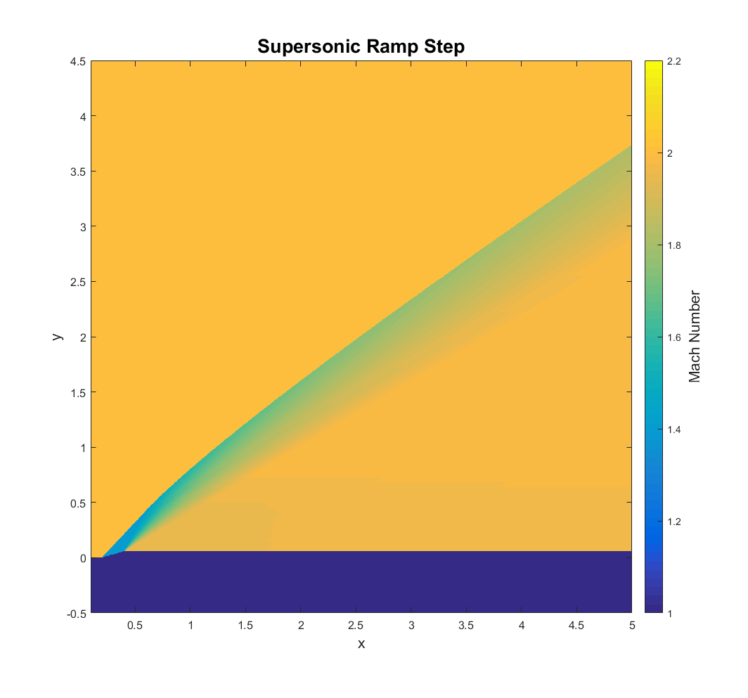
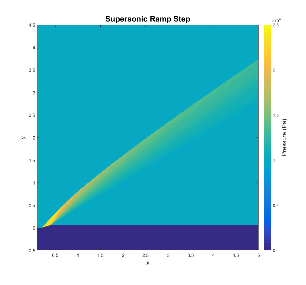
In this case, air enters the domain on the left at Mach 2. The freestream pressure is 10,000 Pascals, the atmospheric pressure at an altitude of about 16,000 meters. The fluid encounters a concave corner, turning the flow 16 degrees and forming a shockwave, across which the Mach number drops to about 1.4 and the static pressure rises to about 23,000 Pascals. Shortly after, a convex corner turns the flow back to its original flow direction, forming a Prandtl-Meyer expansion fan that brings the other flow properties close to their freestream values. The shockwave is then gradually attenuated by the Mach waves of the expansion fan down stream.
The interesting aspect of this case can be seen in the wave plot. It is clear that while most of the expansion waves are absorbed by the shockwave, there is a part of each of them that is reflected. Consider what would happen if there was no reflection. A shockwave and an expansion wave intersect. The fluid below the intersection would pass through a shockwave and an expansion wave while the fluid above the intersection would only pass through a relatively weaker shockwave. Because shockwaves are not isentropic, the stagnation pressure drop below the intersection would be greater than the stagnation pressure drop above the intersection, and consequently, there would generally be a discrepancy in static pressure between the top and bottom regions just after the intersection. To resolve this discrepancy, a reflected expansion wave leaves the point of intersection and the shockwave leaving the point of intersection becomes stronger than it would have been if there was no reflection. The strength of the two waves leaving the intersection are tied together by the flow angle after the intersection, which is solved numerically. This adjustment resolves the pressure discrepancy, but a discrepancy in Mach number known as a slip-line will remain.
The interaction just described is a same-family shock-expansion interaction, meaning that the wave angles are of the same sign relative to the local flow direction. For most same-family interactions, including shock-shock interactions, the reflected wave will usually be relatively weak. For this ramp step case, neglecting the reflections seems to give a surface pressure error of less than 2% freestream pressure. While not a large error, it can perhaps make a difference in moment coefficient calculations or in far field considerations such as shock curvature and sonic boom strength.
Other kinds of interactions are present in the ramp step case, including expansion-slipline interactions and opposite family expansion-expansion interactions. All interactions (and trailing edges) are resolved the same way, with the numerical solution of the flow direction after the intersection point. The one exception is for expansion-expansion interactions, in which a region-to-region method of characteristics can be used instead to decrease computation time. Since this treatment causes the number of waves to grow rapidly, it is usually necessary to include a tolerance where sufficiently weak waves and slip-lines are neglected.
Case 2: The Supersonic Blade Cascade


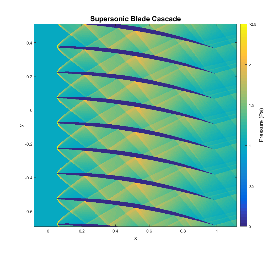
In the design and analysis of axial flow engines, the blade cascade is a useful tool. A set of blades arranged axially around a shaft are “unrolled” and the radial component of velocity is assumed to be much smaller than the axial and tangential components, yielding an effectively two-dimensional flow field around an infinite stack of blade cross-sections. Since the blades are not staggered in this case, this configuration may represent guide vanes, a first stage turbine nozzle, or turbomachinery with a low RPM relative to the axial flow velocity. Generally, the stagnation pressure losses and extreme loading caused by shockwaves has led to the avoidance of supersonic flow in engine design. However, research over the years has demonstrated supersonic turbomachinery can potentially increase power-to-weight ratio enough to offset lower efficiency.
The flow enters from the left at Mach 2 with a pressure of 10,000 Pascals. I have blunted the tips of the blades a bit, giving the leading edge shocks significant curvature initially. This is often done for thermal and structural reasons. The leading edge shocks then bounce between the blades as they slowly dissipate. The air leaves the cascade turned about nine degrees from its inlet value. In this case, I have adjusted the tolerances to neglect all waves reflected from same-family interactions, but the rest can’t be ignored.
It is important to note that, since this is an inviscid analysis, there is no modeling of the boundary layer or its interaction with the shock reflections. With so many shock reflections between the blades, it is likely that there would be significant flow separation if viscosity was considered. No attempt has been made to produce a viable design here. While this kind of analysis could serve as a valuable starting point for a design, this particular example is primarily intended to demonstrate the robustness of the method.
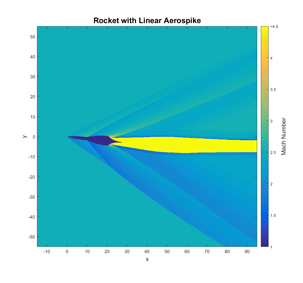
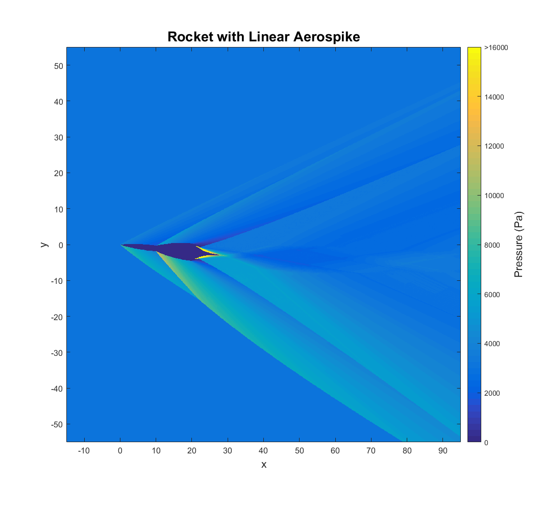
Case 3: The Rocket with Aerospike
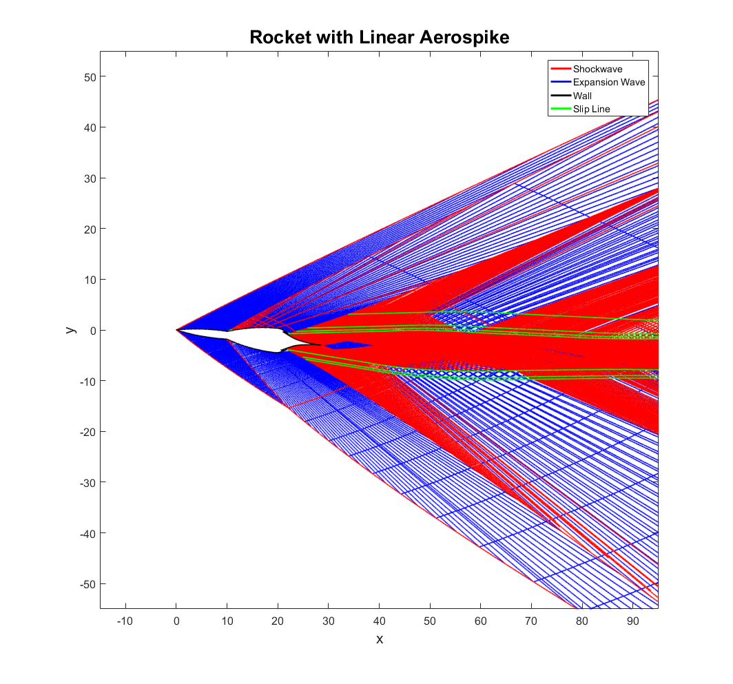
One of the most novel concepts for an altitude compensating rocket engine is the aerospike. If the engine operates at a lower altitude than its designed for, the exhaust is compressed against the spike, providing extra thrust. If the engine operates at a higher altitude than it is designed for, a truncated end with gas injection can be included to extend the effective length of the spike with a region of recirculating flow. This effectively allows the aerospike engine to operate well at any altitude. The drawbacks are that it is mechanically complex and typically heavier than conventional designs. Additionally, its performance suffers a bit at supersonic speeds because the waves around the body effect the exhaust shape.
This particular aerospike is called a linear aerospike. The VentureStar, a space shuttle replacement, was going to use a linear aerospike before the program was canceled. They have the advantages of easier thrust vectoring and a modular design. I have chosen a linear aerospike because the exhaust flow is approximately two-dimensional, one of the assumptions of this method. This also means that the “rocket” it is attached to would need to be more of a spaceplane with a relatively wide lifting body. Truncating the spike would cause a region of subsonic flow to develop, so that detail has been neglected as well. As an added challenge, the vehicle is at a six-degree angle of attack so that the flow field is asymmetric.
The flow enters from the left at Mach 2.5 with a pressure of 3,000 Pascals, atmospheric pressure at an altitude of about 24,000 meters. Shockwaves form on the segmented body and quickly coalesce. The exhaust expands from a pressure of about 5,500,000 Pascals at the throat to about 80,000 Pascals at the end of a conventional diverging nozzle. The exhaust then expands across the spike to a pressure equal to the pressure after the trailing edge shocks, different on top and bottom due to the angle of attack. Moving further down stream, a trail of shock diamonds starts to become visible, especially in the pressure plot. This is because the atmospheric pressure is lower than what this engine is designed for, making it underexpanded. When surrounded by supersonic flow, these waves within the exhaust are partially transmitted through the plume into the surrounding fluid, creating a ripple like effect. Consequently, the shock diamonds die out rapidly compared to a static fire test, where the flow outside the exhaust plume would be able to adjust to its shape upstream. This behavior would perhaps be more clear with a conventional nozzle and a wider view. It is something I may include in a future post. The tolerances here are set so that while most slip-lines are neglected, most waves are considered. Because the wave plot does not show wave strength, the large number of weak waves makes it a bit deceptive here.
One flaw in this analysis is that the exhaust gas is assumed to be calorically perfect and not reacting. In reality, there would likely be many recombination reactions occurring as the exhaust expands that would effect the engine performance. Additionally, while I did use a specific heat ratio of 1.23 in the exhaust to account for the hot combustion products, the large temperature variation would cause this value to change significantly. As with the case of the blade cascade, this case is less of an attempt at a viable design and more of a showcase for this methods merits.
Future Work
There are many improvements I would like to apply to this method. The most fundamental is simply a clean rewrite that utilizes better coding practices. Unanticipated challenges caused me to often use the code as more of an extended calculator than a robust design tool.
Speed improvements could come from a number of places. The biggest one is that the intersections between every active line are currently recalculated every time an interaction is solved. This is completely unnecessary, and fixing this alone may speed up calculations by an order of magnitude. Another way to increase speed would be to treat small shockwaves as isentropic. This would potentially hurt accuracy a bit, but the method of characteristics could then be used to solve more interactions, cutting out the costly numerical flow direction search. For shockwaves that aren’t small, analytical expressions could be used to find the shock angle. When I first tried this I found significant errors were associated with small deflection angles and large Mach numbers, either from rounding errors or perhaps truncation errors from MATLAB trig functions. Regardless, I think the speed benefits are worth another investigation.
Additional improvements include an extension to three dimensions (or at least to axisymmetric flow), variable specific heats, atmospheric effects in the far-field, more parameterized error tolerances, and perhaps a GUI. Beyond these things, this method could certainly benefit from much more verification and validation.
For any questions, comments, or concerns, please feel free to contact me at: daniel@dotsoncentral.com